Mathematics
Gaussian mixed models: covariance, marginal likelihood and shrinkage
1. Students within schools
These are synthetic observations, not real student records. R seed 20261015 generates 250 students in 12 schools with different group sizes. Study hours are uniform from 1 to 12; prior scores are clipped 40 + 3 × hours + normal noise with standard deviation 8, then rounded. Assessment scores follow
\[y_i=50+1.8\,\mathrm{hours}_i+0.2\,\mathrm{prior}_i+b_{g(i)}+\epsilon_i, \quad b_g\sim N(0,6^2),\quad\epsilon_i\sim N(0,5^2).\]
The school effect is shared by students in that school. Conditional on school effects, residual errors are independent. Integrating over those effects makes students within the same school correlated. Scores are continuous, unlike the binary outcomes in logistic/probit or counts in Poisson. Known simulation parameters and estimated parameters are different objects.
from pathlib import Path
import json
import numpy as np
import pandas as pd

from scipy.optimize import brentq
from scipy.stats import norm
from IPython.display import Math, display
ROOT=next(p for p in [Path.cwd(),*Path.cwd().parents] if (p/'Cargo.toml').exists())
import sys
sys.path.insert(0,str(ROOT/'docs/figures'))
from bridge import render_figure
observations=pd.read_csv(ROOT/'docs/data/schools.csv')
X=np.column_stack([np.ones(len(observations)),observations[['study_hours','prior_score']]])
y=observations.score.to_numpy()
labels=list(dict.fromkeys(observations.school))
groups=pd.Categorical(observations.school,categories=labels).codes
members=[np.flatnonzero(groups==g) for g in range(len(labels))]
n,p=X.shape;G=len(members)
fixture=json.loads((ROOT/'tests/fixtures/lmm-r.json').read_text())['cases'][0]
np.testing.assert_array_equal(X,fixture['x']);np.testing.assert_array_equal(y,fixture['y'])
display(observations.head(8))
display(observations[['study_hours','prior_score','score']].corr())
def number(value):
    text = f"{value:.6g}"
    if "e" in text:
        mantissa, exponent = text.split("e")
        return mantissa + rf"\times10^{{{int(exponent)}}}"
    return text

def show_matrix(symbol, values, limit=6):
    matrix = np.asarray(values)
    if matrix.ndim == 1:
        matrix = matrix[:, None]
    indices = list(range(len(matrix))) if len(matrix) <= limit else [0,1,2,None,len(matrix)-1]
    columns = list(range(matrix.shape[1])) if matrix.shape[1] <= limit else [0,1,2,None,matrix.shape[1]-1]
    rows = [" & ".join(r"\ddots" if j is None else r"\vdots" for j in columns) if i is None
            else " & ".join(r"\cdots" if j is None else number(matrix[i,j]) for j in columns) for i in indices]
    display(Math(symbol + r"=\begin{bmatrix}" + r" \\ ".join(rows)
                 + r"\end{bmatrix}" + rf"\quad({matrix.shape[0]}\times{matrix.shape[1]})"))

def show_dot(symbol, left, right):
    terms = [rf"({number(a)})\cdot({number(b)})" for a,b in zip(left,right)]
    if len(terms) > 3:
        terms = terms[:2] + [r"\cdots", terms[-1]]
    display(Math(symbol + "=" + "+".join(terms) + r"\approx" + number(np.asarray(left) @ right)))


show_matrix('X',X);show_matrix('y',y)
Z=np.eye(G)[groups]
show_matrix('Z',Z)
print('Observations:',n,'Fixed coefficients:',p,'Schools:',G)| school | study_hours | prior_score | score | |
|---|---|---|---|---|
| 0 | school-01 | 11.58 | 77.33 | 78.257 |
| 1 | school-01 | 2.70 | 51.70 | 67.242 |
| 2 | school-01 | 10.02 | 78.82 | 88.223 |
| 3 | school-01 | 3.71 | 45.34 | 68.546 |
| 4 | school-01 | 4.38 | 53.50 | 60.137 |
| 5 | school-01 | 5.51 | 71.30 | 72.147 |
| 6 | school-01 | 2.74 | 48.11 | 60.355 |
| 7 | school-01 | 5.21 | 64.25 | 69.670 |
| study_hours | prior_score | score | |
|---|---|---|---|
| study_hours | 1.000000 | 0.775730 | 0.744352 |
| prior_score | 0.775730 | 1.000000 | 0.708543 |
| score | 0.744352 | 0.708543 | 1.000000 |
\(\displaystyle X=\begin{bmatrix}1 & 11.58 & 77.33 \\ 1 & 2.7 & 51.7 \\ 1 & 10.02 & 78.82 \\ \vdots & \vdots & \vdots \\ 1 & 7.33 & 54.19\end{bmatrix}\quad(250\times3)\)
\(\displaystyle y=\begin{bmatrix}78.257 \\ 67.242 \\ 88.223 \\ \vdots \\ 64.224\end{bmatrix}\quad(250\times1)\)
\(\displaystyle Z=\begin{bmatrix}1 & 0 & 0 & \cdots & 0 \\ 1 & 0 & 0 & \cdots & 0 \\ 1 & 0 & 0 & \cdots & 0 \\ \vdots & \vdots & \vdots & \ddots & \vdots \\ 0 & 0 & 0 & \cdots & 1\end{bmatrix}\quad(250\times12)\)
Observations: 250 Fixed coefficients: 3 Schools: 12X and y are observed inputs; ones are a constructed fixed-intercept column. Z is a constructed group-indicator matrix: each row has exactly one 1. Group labels identify membership; they are not numeric predictors. Matrix displays truncate rows/columns using dots while calculations use every observation. Sample correlations alone do not establish causation.
2. Conditional and marginal models
The conditional model is
\[y\mid b\sim N(X\beta+Zb,\sigma^2 I),\qquad b\sim N(0,\tau^2 I_G).\]
Fixed effects beta describe the population relationship. Random intercepts b are modeled as draws from a common zero-mean distribution, not G freely estimated fixed coefficients. sigma² is within-school residual variance; tau² is between-school variance after accounting for X. Normality and independence are modeling assumptions.
Marginalizing over b gives
\[y\sim N(X\beta,V),\qquad V=\sigma^2 I+\tau^2 ZZ^\top.\]
For two different students in the same school, covariance is tau². For different schools it is zero. A single student’s marginal residual variance is sigma² + tau². The intraclass correlation, conditional on fixed predictors, is
\[\mathrm{ICC}=\frac{\tau^2}{\tau^2+\sigma^2}.\]
This is not the raw Pearson correlation of the observed scores. The covariance structure concerns unexplained variation after accounting for fixed effects. For a school of size m,
\[V_g=\sigma^2 I_m+\tau^2\mathbf1\mathbf1^\top.\]
# Display a block using generating variances, not fitted or starting parameters.
m=len(members[0]);Vg=25*np.eye(m)+36*np.ones((m,m))
show_matrix(r'V_{\mathrm{school\ 1}}\text{ at generating parameters}',Vg)
print('Generating ICC:',36/(36+25))
\(\displaystyle V_{\mathrm{school\ 1}}\text{ at generating parameters}=\begin{bmatrix}61 & 36 & 36 & \cdots & 36 \\ 36 & 61 & 36 & \cdots & 36 \\ 36 & 36 & 61 & \cdots & 36 \\ \vdots & \vdots & \vdots & \ddots & \vdots \\ 36 & 36 & 36 & \cdots & 61\end{bmatrix}\quad(18\times18)\)
Generating ICC: 0.59016393442622953. The likelihood integrates out group effects
The marginal Gaussian log-likelihood is
\[\ell(\beta,\sigma^2,\tau^2)=-\frac12\left[ n\log(2\pi)+\log|V|+(y-X\beta)^\top V^{-1}(y-X\beta)\right].\]
This is not a Gaussian likelihood using conditional residuals as independent observations, and not the joint likelihood obtained by treating b as ordinary fixed parameters. It includes the covariance determinant and integrates over b.
For fixed variance components, maximizing over beta gives generalized least squares (GLS):
\[X^\top V^{-1}X\hat\beta=X^\top V^{-1}y.\]
OLS assumes covariance proportional to I. GLS changes how residual directions are weighted because group means and within-group deviations have different variances. The production solve uses whitening and SVD, rather than inverting this cross-product.
4. Whiten groups instead of building a huge matrix
Write rho=tau²/sigma² and C=I+rho ZZ’. For one group,
\[C_g=I_m+\rho\mathbf1\mathbf1^\top,\quad C_g^{-1}=I_m-\frac{\rho}{1+m\rho}\mathbf1\mathbf1^\top,\quad \log|C_g|=\log(1+m\rho).\]
The group-mean direction has eigenvalue 1+m rho; all m-1 directions orthogonal to it have eigenvalue 1. Whitening preserves within-group deviations and divides the mean by sqrt(1+m rho):
\[C_g^{-1/2}v=(v-\bar v\mathbf1)+\frac{\bar v}{\sqrt{1+m\rho}}\mathbf1.\]
This transformation applies to y and each column of X. The squared whitened residual norm is q=(y-X beta)’ C^-1 (y-X beta). It requires storage linear in n, without constructing the full n × n V. Scaling X’s columns as D gives A=XD^-1; weighted SVD solves C^-1/2 A theta approximately C^-1/2 y, with beta=D^-1 theta.
scales=np.linalg.norm(X,axis=0);A=X/scales

def whiten(values,rho):
    matrix=np.asarray(values)
    if matrix.ndim==1:matrix=matrix[:,None]
    output=matrix.copy()
    for indices in members:
        mean=matrix[indices].mean(axis=0)
        output[indices]=(matrix[indices]-mean)+mean/np.sqrt(1+len(indices)*rho)
    return output

rho_trial=1.0
show_matrix(r'C_{g}^{-1}\text{ at trial }\rho=1',np.eye(m)-np.ones((m,m))/(1+m))
show_matrix(r'C^{-1/2}X\text{ at trial }\rho=1',whiten(X,rho_trial))
show_matrix(r'C^{-1/2}y\text{ at trial }\rho=1',whiten(y,rho_trial))
wx=whiten(X,rho_trial);wy=whiten(y,rho_trial)[:,0]
show_dot(r'(X^\top C^{-1}y)_2',wx[:,1],wy)
show_matrix(r'X^\top C^{-1}X\text{ for illustration}',wx.T@wx)
\(\displaystyle C_{g}^{-1}\text{ at trial }\rho=1=\begin{bmatrix}0.947368 & -0.0526316 & -0.0526316 & \cdots & -0.0526316 \\ -0.0526316 & 0.947368 & -0.0526316 & \cdots & -0.0526316 \\ -0.0526316 & -0.0526316 & 0.947368 & \cdots & -0.0526316 \\ \vdots & \vdots & \vdots & \ddots & \vdots \\ -0.0526316 & -0.0526316 & -0.0526316 & \cdots & 0.947368\end{bmatrix}\quad(18\times18)\)
\(\displaystyle C^{-1/2}X\text{ at trial }\rho=1=\begin{bmatrix}0.229416 & 6.49586 & 28.7772 \\ 0.229416 & -2.38414 & 3.1472 \\ 0.229416 & 4.93586 & 30.2672 \\ \vdots & \vdots & \vdots \\ 0.218218 & 2.98486 & 10.9594\end{bmatrix}\quad(250\times3)\)
\(\displaystyle C^{-1/2}y\text{ at trial }\rho=1=\begin{bmatrix}22.0722 \\ 11.0572 \\ 32.0382 \\ \vdots \\ 14.2065\end{bmatrix}\quad(250\times1)\)
\(\displaystyle (X^\top C^{-1}y)_2=(6.49586)\cdot(22.0722)+(-2.38414)\cdot(11.0572)+\cdots+(2.98486)\cdot(14.2065)\approx11169.5\)
\(\displaystyle X^\top C^{-1}X\text{ for illustration}=\begin{bmatrix}11.436 & 75.4292 & 682.398 \\ 75.4292 & 2949.7 & 11782.4 \\ 682.398 & 11782.4 & 76897.9\end{bmatrix}\quad(3\times3)\)
Trial rho is a starting/example variance ratio, not an observed predictor or a known generating parameter. The cross-product shown is for understanding the dot products; production estimation uses the SVD of an equivalent compact weighted design, derived next.
Cache a square-root reduction, following the lme4 idea
lme4 evaluates a penalized least-squares problem and eliminates the random coefficients through a block factorization. For our single random intercept, the same elimination has a particularly simple form. At positive rho,
\[\min_b\left\{\sum_{i\in g}(r_i-b)^2+\frac{b^2}{\rho}\right\} =\sum_{i\in g}(r_i-\bar r_g)^2+\frac{m_g\bar r_g^2}{1+m_g\rho}.\]
The minimizer is \(b=m_g\rho\bar r_g/(1+m_g\rho)\); substitute it into the left side to obtain the right side. At rho=0 the limiting solution has b=0. Within-group deviations have weight 1; only the group-mean weight changes with the variance ratio. This is the link between penalized least squares and the marginal GLS residual norm above.
We can therefore do most observation-level work once. Let W contain within-group-centered rows of the augmented matrix \([A\;y]\), and let row g of M be \(\sqrt{m_g}[\bar A_g\;\bar y_g]\). Take a thin QR factorization \(W=Q_wR_w\). Since \(Q_w^\top Q_w=I\), for any coefficient vector theta,
\[q(\rho,\theta)=\left\|W\begin{bmatrix}-\theta\\1\end{bmatrix}\right\|^2 +\sum_g\frac{\left(M_g\begin{bmatrix}-\theta\\1\end{bmatrix}\right)^2}{1+m_g\rho} =\left\|K(\rho)\begin{bmatrix}-\theta\\1\end{bmatrix}\right\|^2,\]
\[K(\rho)=\begin{bmatrix}R_w\\ \operatorname{diag}\{(1+m_g\rho)^{-1/2}\}M\end{bmatrix}.\]
K has only p+1+G rows. The fixed intercept’s centered column is zero; that poses no problem for QR of the augmented matrix. Full rank is checked on the complete weighted fixed design, including the group-mean rows.
augmented=np.column_stack([A,y])
centered=augmented.copy();means=[];sizes=np.array([len(rows) for rows in members])
for rows in members:
    mean=augmented[rows].mean(axis=0)
    centered[rows]=augmented[rows]-mean
    means.append(np.sqrt(len(rows))*mean)
means=np.asarray(means)
_,within_R=np.linalg.qr(centered,mode='reduced')
compact=np.vstack([within_R,means/np.sqrt(1+sizes[:,None]*rho_trial)])
show_matrix(r'R_w',within_R)
show_matrix(r'K(\rho=1)',compact)
trial_theta=np.array([40.,1.,.1])*scales
contrast=np.r_[-trial_theta,1.]
compressed_q=np.linalg.norm(compact@contrast)**2
full_q=np.linalg.norm(whiten(y-X@(trial_theta/scales),rho_trial))**2
np.testing.assert_allclose(compressed_q,full_q,atol=1e-8,rtol=1e-12)
print('Original rows:',n,'Compact rows:',len(compact))
print('Trial residual norm squared: full =',full_q,'compact =',compressed_q)
compressed_beta=np.linalg.lstsq(compact[:,:p],compact[:,p],rcond=None)[0]/scales
full_beta=np.linalg.lstsq(whiten(A,rho_trial),whiten(y,rho_trial)[:,0],rcond=None)[0]/scales
np.testing.assert_allclose(compressed_beta,full_beta,atol=1e-9,rtol=1e-10)
show_matrix(r'\hat\beta(\rho=1)\text{ from compact solve}',compressed_beta)
\(\displaystyle R_w=\begin{bmatrix}-2.19427\times10^{-16} & 2.37666\times10^{-17} & -9.24052\times10^{-18} & 8.03564\times10^{-14} \\ 0 & 0.425853 & 0.152078 & 115.712 \\ 0 & 0 & -0.124809 & -29.3396 \\ 0 & 0 & 0 & -77.6791\end{bmatrix}\quad(4\times4)\)
\(\displaystyle K(\rho=1)=\begin{bmatrix}-2.19427\times10^{-16} & 2.37666\times10^{-17} & -9.24052\times10^{-18} & 8.03564\times10^{-14} \\ 0 & 0.425853 & 0.152078 & 115.712 \\ 0 & 0 & -0.124809 & -29.3396 \\ \vdots & \vdots & \vdots & \vdots \\ 0.0617213 & 0.0466966 & 0.0559028 & 62.4369\end{bmatrix}\quad(16\times4)\)
Original rows: 250 Compact rows: 16
Trial residual norm squared: full = 13535.464479982495 compact = 13535.464479982504
\(\displaystyle \hat\beta(\rho=1)\text{ from compact solve}=\begin{bmatrix}46.6818 \\ 1.61463 \\ 0.244911\end{bmatrix}\quad(3\times1)\)
Production caches R_w and M once, then uses SVD on the compact weighted fixed design. Covariance is computed only at the selected fit. The later Python profile deliberately uses the full whitening formulation as an independent check of the same mathematics. For a million observations and 100 groups with three coefficients, each trial now factors 104 rows instead of a million.
This borrows elimination and reuse from lme4; it does not copy lme4 source code or introduce its sparse Cholesky/CHOLMOD backend. Using QR/SVD square roots also avoids subtracting nearly equal Gram matrices or forming a residual norm as \(y^\top y-\hat\beta^\top X^\top y\). That preserves accuracy with correlated predictors and small residual variation. See lme4’s PLS versus GLS derivation and the measured optimization.
5. Profile out beta and sigma²; optimize one variance ratio
At fixed rho, GLS finds beta and q. The ML scale estimate is
\[\hat\sigma^2(\rho)=q(\rho)/n,\qquad\hat\tau^2=\rho\hat\sigma^2.\]
Substitution gives the profiled negative log-likelihood
\[f(\rho)=\frac12\left[n\{\log(2\pi)+1+\log(q/n)\} +\sum_g\log(1+m_g\rho)\right].\]
A lower value is better. No generic multivariate optimizer is required for this particular random-intercept model. For GLS residuals r=y-X beta, the envelope theorem lets us differentiate the optimized objective without differentiating beta:
\[q'(\rho)=-\sum_g\frac{(\sum_{i\in g}r_i)^2}{(1+m_g\rho)^2},\qquad f'(\rho)=\frac12\left[n\frac{q'}q+\sum_g\frac{m_g}{1+m_g\rho}\right].\]
Rust searches t=log(1+rho) on a 0.5-spaced grid from 0 to 32, then refines every negative-to-positive derivative crossing by 40 bisections. The derivative with respect to t is (1+rho)f’(rho). It compares those candidates with rho=0 exactly, and rejects an optimum beyond the upper bound. The finite grid can miss unusually narrow unbracketed stationary points: this initial search is not an exhaustive global-optimum guarantee. The Python walkthrough independently brackets roots of the same score, using SciPy’s root solver.
def profile(t):
    rho=np.expm1(t);wx=whiten(A,rho);wy=whiten(y,rho)[:,0]
    U,s,Vt=np.linalg.svd(wx,full_matrices=False)
    beta=(Vt.T@((U.T@wy)/s))/scales
    residual=y-X@beta
    q=np.sum(whiten(residual,rho)**2);variance=q/n
    logdet=sum(np.log1p(len(indices)*rho) for indices in members)
    objective=.5*(n*(np.log(2*np.pi)+1+np.log(variance))+logdet)
    qprime=-sum((residual[indices].sum()/(1+len(indices)*rho))**2 for indices in members)
    derivative=.5*(1+rho)*(n*qprime/q+sum(len(indices)/(1+len(indices)*rho) for indices in members))
    return dict(rho=rho,beta=beta,variance=variance,objective=objective,derivative=derivative,s=s,Vt=Vt)

grid=np.arange(0,32.5,.5);values=[profile(t) for t in grid];candidates=[0.]
for left,right,a,b in zip(grid[:-1],grid[1:],values[:-1],values[1:]):
    if a['derivative']<0 and b['derivative']>=0:
        candidates.append(brentq(lambda t:profile(t)['derivative'],left,right,xtol=1e-12))
best_t=min(candidates,key=lambda t:profile(t)['objective'])
fit=profile(best_t);rho=fit['rho'];beta=fit['beta'];variance=fit['variance'];tau=rho*variance
print('Candidate log ratios:',candidates)
print('Residual variance:',variance,'Group variance:',tau,'ICC:',rho/(1+rho))
show_matrix(r'\hat\beta',beta)

curve=np.linspace(0,4,81);objective=np.array([profile(t)['objective'] for t in curve])
render_figure('profile',dict(curve=curve.tolist(),objective=(objective-objective.min()).tolist(),
                           best_t=float(best_t),boundary=float(profile(0)['objective']-objective.min())))
Candidate log ratios: [0.0, 0.538861158638389]
Residual variance: 25.355429364972306 Group variance: 18.105138532639522 ICC: 0.4165877117688194\(\displaystyle \hat\beta=\begin{bmatrix}46.6552 \\ 1.61391 \\ 0.245431\end{bmatrix}\quad(3\times1)\)
figures/lmm-profile.svg 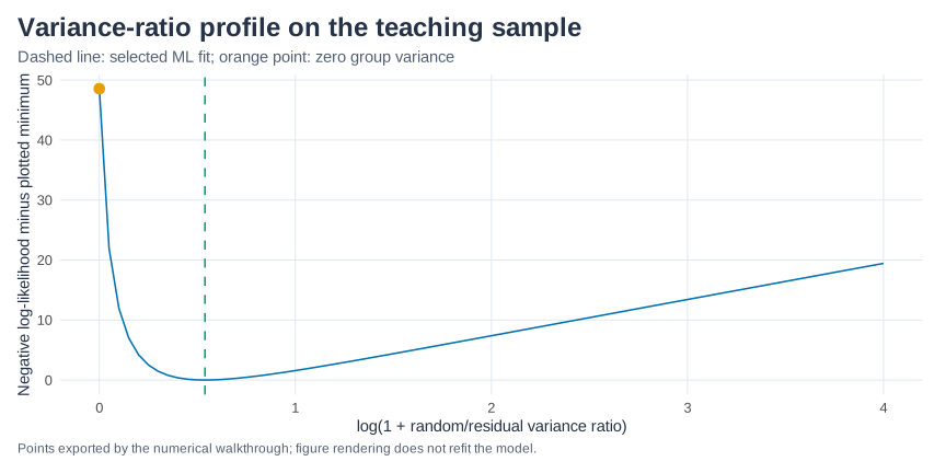
ML is not REML. Restricted maximum likelihood adjusts for estimating fixed coefficients and adds a fixed-design determinant term; it often improves variance estimation with limited groups. R lmer defaults to REML, so all comparisons here explicitly set REML=FALSE. No RSS/(n-p) correction is substituted for the ML scale.
6. Shrinkage: estimate each school’s intercept
At the fitted variances, the Gaussian conditional mean of a group effect is
\[\hat b_g=\frac{m_g\hat\tau^2}{\hat\sigma^2+m_g\hat\tau^2}\bar r_g, \qquad\bar r_g=\frac1{m_g}\sum_{i\in g}(y_i-x_i^\top\hat\beta).\]
To derive it, combine the prior term b²/tau² with the within-group likelihood sum(r_i-b)²/sigma². The resulting quadratic in b has precision 1/tau² + m/sigma² and linear term sum r_i/sigma², yielding this conditional mean. The multiplier lies between 0 and 1: noisy/small groups shrink more toward zero. These empirical BLUPs use fitted variances; they are not known realized effects. At tau²=0 all group effects are zero.
fixed_fitted=X@beta;marginal_residuals=y-fixed_fitted
random_effects=np.array([(len(indices)*rho/(1+len(indices)*rho))*marginal_residuals[indices].mean() for indices in members])
fitted=fixed_fitted+random_effects[groups];residuals=y-fitted
summary=pd.DataFrame({'school':labels,'n':[len(i) for i in members],
                     'raw residual mean':[marginal_residuals[i].mean() for i in members],
                     'shrinkage':[len(i)*rho/(1+len(i)*rho) for i in members],
                     'estimated random intercept':random_effects})
display(summary)
show_dot(r'x_1^\top\hat\beta',X[0],beta)
display(pd.DataFrame({'observed':y,'population fit':fixed_fitted,'conditional fit':fitted,
'marginal residual':marginal_residuals,'conditional residual':residuals}).head(8))| school | n | raw residual mean | shrinkage | estimated random intercept | |
|---|---|---|---|---|---|
| 0 | school-01 | 18 | 0.144569 | 0.927813 | 0.134133 |
| 1 | school-02 | 24 | 1.702569 | 0.944865 | 1.608698 |
| 2 | school-03 | 15 | -1.951292 | 0.914609 | -1.784668 |
| 3 | school-04 | 22 | -5.918576 | 0.940153 | -5.564365 |
| 4 | school-05 | 20 | 0.266511 | 0.934560 | 0.249070 |
| 5 | school-06 | 27 | 2.373478 | 0.950689 | 2.256439 |
| 6 | school-07 | 19 | 11.092734 | 0.931352 | 10.331238 |
| 7 | school-08 | 21 | -5.445123 | 0.937481 | -5.104699 |
| 8 | school-09 | 16 | 2.286798 | 0.919516 | 2.102748 |
| 9 | school-10 | 25 | 0.600960 | 0.946953 | 0.569081 |
| 10 | school-11 | 23 | 0.083845 | 0.942605 | 0.079033 |
| 11 | school-12 | 20 | -5.218187 | 0.934560 | -4.876707 |
\(\displaystyle x_1^\top\hat\beta=(1)\cdot(46.6552)+(11.58)\cdot(1.61391)+(77.33)\cdot(0.245431)\approx84.3234\)
| observed | population fit | conditional fit | marginal residual | conditional residual | |
|---|---|---|---|---|---|
| 0 | 78.257 | 84.323391 | 84.457524 | -6.066391 | -6.200524 |
| 1 | 67.242 | 63.701502 | 63.835635 | 3.540498 | 3.406365 |
| 2 | 88.223 | 82.171386 | 82.305519 | 6.051614 | 5.917481 |
| 3 | 68.546 | 63.770610 | 63.904743 | 4.775390 | 4.641257 |
| 4 | 60.137 | 66.854642 | 66.988775 | -6.717642 | -6.851775 |
| 5 | 72.147 | 73.047023 | 73.181156 | -0.900023 | -1.034156 |
| 6 | 60.355 | 62.884962 | 63.019095 | -2.529962 | -2.664095 |
| 7 | 69.670 | 70.832565 | 70.966698 | -1.162565 | -1.296698 |
The population fit describes a group with mean effect zero. The conditional fit uses this sample’s estimated group effect. It is not a held-out predictive result: the same outcomes helped estimate those effects. There is no new-group prediction API.
7. Fixed-effect uncertainty and model statistics
The plug-in GLS covariance is
\[\widehat{\operatorname{Var}}(\hat\beta)=(X^\top\hat V^{-1}X)^{-1} =\hat\sigma^2 D^{-1}VS^{-2}V^\top D^{-1},\]
where V and S on the right are the SVD factors of the whitened scaled design (the SVD factor V is distinct from the observation covariance V). Standard errors are diagonal square roots. We report asymptotic normal Wald z-tests and intervals. There is no exact OLS t distribution, Satterthwaite/Kenward–Roger adjustment or variance-component p-value. With only twelve groups, normal inference should be read cautiously: many students do not substitute for many independent groups.
AIC uses p+2 parameters: fixed coefficients and both variance components, counting them even when tau²=0. Group BLUPs are not counted as G additional free parameters. The returned df_residual=n-p is informational, not a t-test denominator.
s=fit['s'];Vt=fit['Vt']
covariance=variance*((Vt.T/s)@(Vt/s[:,None]))/scales[:,None]/scales[None,:]
se=np.sqrt(np.diag(covariance));z=beta/se;p_values=2*norm.sf(abs(z))
conf_int=np.column_stack([beta-norm.ppf(.975)*se,beta+norm.ppf(.975)*se])
display(pd.DataFrame({'estimate':beta,'SE':se,'z':z,'p':p_values,'95% lower':conf_int[:,0],'95% upper':conf_int[:,1]},index=['intercept','study hours','prior score']))
calculated=dict(coefficients=beta,covariance=covariance,std_errors=se,z_statistics=z,p_values=p_values,conf_int=conf_int,
 fixed_fitted=fixed_fitted,fitted=fitted,residuals=residuals,marginal_residuals=marginal_residuals,random_effects=random_effects,
 residual_variance=variance,random_intercept_variance=tau,sigma=np.sqrt(variance),icc=rho/(1+rho),
 log_likelihood=-fit['objective'],aic=2*(p+2)+2*fit['objective'],df_residual=n-p)
for key,value in calculated.items():
    np.testing.assert_allclose(value,fixture['reference']['result'][key],atol=1e-7,rtol=1e-6,err_msg=key)
print('Every statistical field agrees with the saved lme4 ML fixture.')| estimate | SE | z | p | 95% lower | 95% upper | |
|---|---|---|---|---|---|---|
| intercept | 46.655187 | 2.204067 | 21.167768 | 1.893113e-99 | 42.335294 | 50.975079 |
| study hours | 1.613908 | 0.160247 | 10.071362 | 7.394690e-24 | 1.299829 | 1.927987 |
| prior score | 0.245431 | 0.041713 | 5.883790 | 4.009775e-09 | 0.163675 | 0.327187 |
Every statistical field agrees with the saved lme4 ML fixture.8. Boundaries, assumptions and experiments
A zero random-intercept variance is a valid boundary ML fit. It gives OLS fixed coefficients but uses the ML scale RSS/n for standard errors, rather than OLS’s unbiased RSS/(n-p). Positive residual variance is required; numerically perfect fits and unsupported zero-residual-variance limits fail. One group or all-singleton data are rejected because the two variances cannot be separately identified under this first contract; singleton groups are allowed when other groups repeat.
Assumptions include independent groups, Gaussian random intercepts independent of X, homoskedastic Gaussian residuals and the supplied linear fixed mean. Ignoring correlation between random effects and predictors can bias fixed effects. The first implementation has one grouping factor, no random slopes or REML. Missing rows in x, y or groups are deleted together, with warnings and row metadata.
Try merging all groups into one; assigning each row a new group; removing the school variation in the simulation; or increasing residual noise. Which makes the model unidentified, pushes group variance to zero, or increases shrinkage?
Rust connections
fit_random_intercept owns numeric vectors and usize group IDs. A HashMap assigns first-appearance group indices; vectors of member row positions make group means and group means explicit. ProfileData caches a QR square-root summary and group means; a private Profile struct holds one variance-ratio evaluation. nalgebra’s SVD handles compact GLS and final covariance; the dedicated scalar search remains visible in crates/stats-core/src/mixed.rs. Result/? propagates validation and numerical errors. The binding preserves typed PHP group labels, handles missing rows and converts the complete result to ordinary arrays.
See the PHP contract, executed comparison, lme4 lmer reference, and statsmodels MixedLM.
From phpstats/phit@76b22f0.