Mathematics
Binomial mixed models: likelihood, latent effects and integration
We now model a binary or grouped-binomial outcome with a Gaussian random intercept. The outcome distribution changes; the group-effect distribution remains Gaussian. This walkthrough uses the published cattle-disease cbpp data from lme4, with 56 herd/period records across 15 herds. Period one is the baseline. Data source: Lesnoff et al. (2004), Preventive Veterinary Medicine 64, 27–40. The CSV, provenance/checksum and license are included in the site.
Observed counts and constructed predictors
\[ s_i\mid b_{g(i)}\sim\operatorname{Binomial}(m_i,p_i),\qquad \eta_i=o_i+x_i^\top\beta+b_{g(i)},\qquad p_i=\frac{1}{1+e^{-\eta_i}}. \]
Here s is the observed number of new cases and m the number of animals at risk. The API takes y=s/m and weights=m; m=1 gives ordinary binary observations. The known offset o is zero in this example. The fixed columns are ones and indicators for observed periods 2, 3 and 4. These are data/prepared predictors, not guesses at coefficients.
from pathlib import Path
import json,sys
import numpy as np
import pandas as pd

from scipy.special import expit,logsumexp
from scipy.optimize import brentq
from scipy.integrate import quad
from scipy.linalg import cho_factor,cho_solve
from IPython.display import display,Math
ROOT=next(p for p in [Path.cwd(),*Path.cwd().parents] if (p/'Cargo.toml').exists())
import sys
sys.path.insert(0,str(ROOT/'docs/figures'))
from bridge import render_figure
sys.path.insert(0,str(ROOT/'docs/verifications'))
from compare_logistic_mixed import evaluator
fixture=json.loads((ROOT/'tests/fixtures/logistic-mixed-r.json').read_text())
report=json.loads((ROOT/'docs/verifications/logistic-mixed-results.json').read_text())
c=next(c for c in fixture['cases'] if c['name']=='cbpp_61')
fit=next(r['PHP'] for r in report['results'] if r['name']==c['name'])
raw=pd.read_csv(ROOT/'docs/data/cbpp.csv');display(raw.head(8))
x=np.array(c['x']);y=np.array(c['y']);m=np.array(c['weights']);s=np.round(y*m);groups=np.array(c['groups'])
beta=np.array(fit['coefficients']);tau=fit['random_intercept_sd']
def matrix(a,name):
    a=np.atleast_2d(a)
    body=r' \\ '.join(' & '.join(f'{v:.6g}' for v in row) for row in a)
    display(Math(name+r'=\begin{bmatrix}'+body+r'\end{bmatrix}'))
ids=np.flatnonzero(groups==groups[0]);display(raw.iloc[ids])
matrix(x[ids],r'X_{\mathrm{first\ herd}}')
matrix(beta[:,None],r'\hat\beta')
matrix((x[ids]@beta)[:,None],r'X_g\hat\beta')
print('X shape:',x.shape,'group count:',len(set(groups)))| herd | incidence | size | period | |
|---|---|---|---|---|
| 0 | 1 | 2 | 14 | 1 |
| 1 | 1 | 3 | 12 | 2 |
| 2 | 1 | 4 | 9 | 3 |
| 3 | 1 | 0 | 5 | 4 |
| 4 | 2 | 3 | 22 | 1 |
| 5 | 2 | 1 | 18 | 2 |
| 6 | 2 | 1 | 21 | 3 |
| 7 | 3 | 8 | 22 | 1 |
| herd | incidence | size | period | |
|---|---|---|---|---|
| 0 | 1 | 2 | 14 | 1 |
| 1 | 1 | 3 | 12 | 2 |
| 2 | 1 | 4 | 9 | 3 |
| 3 | 1 | 0 | 5 | 4 |
\(\displaystyle X_{\mathrm{first\ herd}}=\begin{bmatrix}1 & 0 & 0 & 0 \\ 1 & 1 & 0 & 0 \\ 1 & 0 & 1 & 0 \\ 1 & 0 & 0 & 1\end{bmatrix}\)
\(\displaystyle \hat\beta=\begin{bmatrix}-1.39923 \\ -0.991404 \\ -1.12782 \\ -1.57947\end{bmatrix}\)
\(\displaystyle X_g\hat\beta=\begin{bmatrix}-1.39923 \\ -2.39063 \\ -2.52705 \\ -2.9787\end{bmatrix}\)
X shape: (56, 4) group count: 15Matrix multiplication takes each observed row’s dot product with beta. The result is log odds, not a probability. The inverse-logit converts it to a probability; adding a herd effect shifts those log odds before conversion.
Conditional likelihood and random-effect law
For one observation,
\[ \log f(s_i\mid b)=\log {m_i\choose s_i} +s_i\eta_i-m_i\log(1+e^{\eta_i}). \]
We specify b_g~N(0,tau²). Write b_g=tau*u_g with u_g~N(0,1), so zero tau is a valid boundary without computing log(0). The fixed coefficients and tau are estimated by marginal maximum likelihood:
\[ L(\beta,\tau)=\prod_g\int \left\{\prod_{i\in g}f(s_i\mid u_g;\beta,\tau)\right\} \phi(u_g)\,du_g. \]
We integrate over unobserved group effects. Merely finding their best values and ignoring this integral would fit a different objective. No prior is placed on beta or tau in this implementation; the Gaussian distribution describes population variation among groups.
Find each conditional mode
Apart from constants independent of u, the log integrand is
\[ k_g(u)=\sum_{i\in g}\{s_i\eta_i-m_i\log(1+e^{\eta_i})\}-\tfrac12u^2. \]
Its score and negative curvature are
\[ k'_g(u)=\tau\sum_{i\in g}(s_i-m_ip_i)-u,\qquad h_g(u)=-k''_g(u)=1+\tau^2\sum_{i\in g}m_ip_i(1-p_i). \]
The prior contributes the 1, making the log integrand strictly concave: every group has a unique conditional mode, even when all its outcomes are failures or successes. Safeguarded Newton updates use u + score/h; a bracket prevents an oversized step from escaping the root.
e=x[ids]@beta;yg=y[ids];mg=m[ids]
def kernel(u):
    eta=e+tau*u
    return -.5*u*u-np.sum(mg*(yg*np.logaddexp(0,-eta)+(1-yg)*np.logaddexp(0,eta)))
mode=brentq(lambda u:tau*np.sum(mg*(yg-expit(e+tau*u)))-u,-20,20,xtol=1e-13)
p=expit(e+tau*mode);h=1+tau*tau*np.sum(mg*p*(1-p))
display(pd.DataFrame(dict(period=raw.iloc[ids].period,successes=s[ids],trials=mg,
                         fixed_log_odds=e,conditional_log_odds=e+tau*mode,
                         probability=p,score_contribution=s[ids]-mg*p,
                         information_contribution=mg*p*(1-p))))
print('Conditional standardized mode:',mode)
print('Random intercept b=tau*u:',tau*mode)
print('Score at mode:',tau*np.sum(mg*(yg-p))-mode)
print('Posterior precision:',h)
assert np.isclose(tau*mode,fit['random_effects'][0],atol=1e-7)| period | successes | trials | fixed_log_odds | conditional_log_odds | probability | score_contribution | information_contribution | |
|---|---|---|---|---|---|---|---|---|
| 0 | 1 | 2.0 | 14 | -1.399230 | -0.806206 | 0.308700 | -2.321795 | 2.987658 |
| 1 | 2 | 3.0 | 12 | -2.390634 | -1.797609 | 0.142142 | 1.294292 | 1.463255 |
| 2 | 3 | 4.0 | 9 | -2.527050 | -1.934025 | 0.126306 | 2.863248 | 0.993173 |
| 3 | 4 | 0.0 | 5 | -2.978701 | -2.385676 | 0.084271 | -0.421357 | 0.385849 |
Conditional standardized mode: 0.9158422853016355
Random intercept b=tau*u: 0.5930248216942333
Score at mode: -8.537615059367454e-14
Posterior precision: 3.444376591207904
Returned random_effects are these conditional modes. With a non-Gaussian outcome, the conditional distribution can be skewed, so its mean and mode need not coincide. Gaussian mixed models have coincident means/modes.
Laplace approximation: use height and curvature
Approximating k by a quadratic near its mode gives
\[ \log L_g\approx\sum_{i\in g}\log{m_i\choose s_i} +k_g(\hat u_g)-\tfrac12\log h_g. \]
The Gaussian prior’s normalization cancels the quadratic integral’s sqrt(2*pi). The curvature term is essential: a narrow peak has less probability mass than a wide peak of the same height. This is the default one-node approximation, matching lme4 glmer(nAGQ=1).
Adaptive Gauss-Hermite quadrature
Let z_j,w_j integrate expectations under N(0,1). Center and scale those nodes at the conditional mode: u_j=mode+z_j/sqrt(h). Then
\[ L_g\approx\left\{\prod_{i\in g}{m_i\choose s_i}\right\} \frac{1}{\sqrt{h_g}}\sum_jw_j \exp\{k_g(u_j)+z_j^2/2\}. \]
For one node z=0,w=1, this is exactly Laplace. More nodes examine the shape away from the peak. We evaluate the sum with log-sum-exp to avoid underflow.
z,w=np.polynomial.hermite_e.hermegauss(9);w/=np.sqrt(2*np.pi)
u=mode+z/np.sqrt(h)
display(pd.DataFrame(dict(normal_node=z,normal_weight=w,adaptive_node=u,
                         log_integrand=[kernel(v) for v in u],
                         corrected_log_term=[np.log(weight)+kernel(v)+node*node/2 for node,weight,v in zip(z,w,u)])))
print('Laplace group log integral, without binomial constant:',kernel(mode)-.5*np.log(h))
print('9-node group log integral, without binomial constant:',
logsumexp([np.log(weight)+kernel(v)+node*node/2 for node,weight,v in zip(z,w,u)])-.5*np.log(h))| normal_node | normal_weight | adaptive_node | log_integrand | corrected_log_term | |
|---|---|---|---|---|---|
| 0 | -4.512746 | 0.000022 | -1.515721 | -32.063604 | -32.590037 |
| 1 | -3.205429 | 0.002789 | -0.811311 | -28.239328 | -28.983962 |
| 2 | -2.076848 | 0.049916 | -0.203207 | -25.779589 | -26.620346 |
| 3 | -1.023256 | 0.244098 | 0.364490 | -24.323492 | -25.210153 |
| 4 | 0.000000 | 0.406349 | 0.915842 | -23.824460 | -24.725002 |
| 5 | 1.023256 | 0.244098 | 1.467194 | -24.372600 | -25.259261 |
| 6 | 2.076848 | 0.049916 | 2.034892 | -26.184028 | -27.024784 |
| 7 | 3.205429 | 0.002789 | 2.642995 | -29.686167 | -30.430801 |
| 8 | 4.512746 | 0.000022 | 3.347405 | -35.920827 | -36.447260 |
Laplace group log integral, without binomial constant: -24.442831257056472
9-node group log integral, without binomial constant: -24.439110716121473
The Rust code gets nodes from eigenvalues of the Hermite Jacobi matrix, whose neighboring entries are sqrt(1), sqrt(2), etc. At 61 nodes, tiny eigenvector components gave insufficient relative accuracy for tail weights. We instead compute weights using the orthonormal polynomial sum w=1/sum(p_k(z)^2). An independent regression test verifies a tail weight of approximately 9.37e-47. Moment checks alone did not expose that tail problem.
Fixed-effect uncertainty comes from the marginal objective
The optimizer searches beta and tau jointly. Each objective evaluation solves all conditional modes and integrates the group effects. Fixed-effect covariance uses the beta block of the inverse joint observed information of the chosen approximate marginal likelihood. It includes coupling to estimated tau; it is not simply the inverse conditional X’WX matrix.
likelihood=evaluator(c);theta=np.r_[beta,tau]
def information(step):
    delta=step*(1+abs(theta));n=len(theta);H=np.zeros((n,n))
    objective=lambda t:-likelihood(t[:-1],t[-1],61)[0]
    f0=objective(theta)
    for i in range(n):
        a=theta.copy();b=theta.copy();a[i]+=delta[i];b[i]-=delta[i]
        H[i,i]=(objective(a)+objective(b)-2*f0)/delta[i]**2
        for j in range(i):
            pp=theta.copy();pm=theta.copy();mp=theta.copy();mm=theta.copy()
            pp[i]+=delta[i];pp[j]+=delta[j];pm[i]+=delta[i];pm[j]-=delta[j]
            mp[i]-=delta[i];mp[j]+=delta[j];mm[i]-=delta[i];mm[j]-=delta[j]
            H[i,j]=H[j,i]=(objective(pp)-objective(pm)-objective(mp)+objective(mm))/(4*delta[i]*delta[j])
    return H
H=(4*information(5e-4)-information(1e-3))/3
cov=cho_solve(cho_factor(H),np.eye(len(theta)))[:-1,:-1]
matrix(H,r'H_{\beta,\tau}')
matrix(cov,r'\widehat{\mathrm{Var}}(\hat\beta)')
print('Standard errors:',np.sqrt(cov.diagonal()))
assert np.allclose(cov,fit['covariance'],atol=1e-6,rtol=1e-4)
\(\displaystyle H_{\beta,\tau}=\begin{bmatrix}23.7642 & 4.62385 & 3.87182 & 1.97006 & 3.45619 \\ 4.62385 & 12.8048 & -1.9477 & -0.981137 & -0.614388 \\ 3.87182 & -1.9477 & 11.0386 & -0.798949 & -0.429364 \\ 1.97006 & -0.981137 & -0.798949 & 6.03101 & -0.393058 \\ 3.45619 & -0.614388 & -0.429364 & -0.393058 & 31.6822\end{bmatrix}\)
\(\displaystyle \widehat{\mathrm{Var}}(\hat\beta)=\begin{bmatrix}0.0545277 & -0.0259514 & -0.025858 & -0.0259234 \\ -0.0259514 & 0.0941066 & 0.0279311 & 0.0278374 \\ -0.025858 & 0.0279311 & 0.106778 & 0.0274714 \\ -0.0259234 & 0.0278374 & 0.0274714 & 0.182837\end{bmatrix}\)
Standard errors: [0.23351159 0.30676799 0.32676837 0.4275945 ]The implementation uses centered finite differences with Richardson extrapolation, then a Cholesky solve. Nonpositive information, nonstationary solutions and exhausted optimizer budgets fail explicitly. Standard errors, z tests and 95% normal Wald intervals are asymptotic approximations. There are no random-variance intervals, finite-group t corrections or REML in this binomial fitter.
Approximation accuracy: a rare-event example
The verification includes independent QUADPACK integration, which does not use Hermite nodes. On the rare-event sample, Laplace and R agree but the fitted group SD differs substantially from higher-node estimation. This is an approximation issue, not a disagreement between implementations.
rare=[r for r in report['results'] if r['dataset']=='rare_events']
display(pd.DataFrame([dict(nodes=r['quadrature_points'],intercept=r['PHP']['coefficients'][0],
                          group_SD=r['PHP']['random_intercept_sd'],
                          approximate_log_likelihood=r['PHP']['log_likelihood'],
                          independently_integrated_log_likelihood=r['scipy_integrated_log_likelihood'],
                          approximation_error=r['approximation_log_likelihood_error']) for r in rare]))
# Compare posterior shape with the Gaussian approximation in a small group.
rc=next(c for c in fixture['cases'] if c['name']=='rare_events_61')
rf=next(r['PHP'] for r in rare if r['quadrature_points']==61)
rx=np.array(rc['x']);ry=np.array(rc['y']);rg=np.array(rc['groups']);rtau=rf['random_intercept_sd'];re=rx@np.array(rf['coefficients'])
choices=[]
for group in dict.fromkeys(rg):
    ids=rg==group;ee=re[ids];yy=ry[ids]
    k=lambda u,ee=ee,yy=yy:-.5*u*u-np.sum(yy*np.logaddexp(0,-ee-rtau*u)+(1-yy)*np.logaddexp(0,ee+rtau*u))
    uu=brentq(lambda u:rtau*np.sum(yy-expit(ee+rtau*u))-u,-30,30)
    hh=1+rtau*rtau*np.sum(expit(ee+rtau*uu)*expit(-ee-rtau*uu))
    norm=quad(lambda u:np.exp(k(u)-k(uu)),-np.inf,np.inf,epsabs=1e-11)[0]
    error=k(uu)-.5*np.log(hh)-(k(uu)+np.log(norm)-.5*np.log(2*np.pi))
    choices.append((abs(error),group,k,uu,hh,norm))
_,group,k,uu,hh,norm=max(choices,key=lambda v:v[0])
u=np.linspace(-4,4,400)
actual=np.array([np.exp(k(v)-k(uu))/norm for v in u]);gaussian=np.sqrt(hh/(2*np.pi))*np.exp(-.5*hh*(u-uu)**2)
render_figure('posterior',dict(u=u.tolist(),actual=actual.tolist(),gaussian=gaussian.tolist(),
mode=float(uu),group=int(group)))| nodes | intercept | group_SD | approximate_log_likelihood | independently_integrated_log_likelihood | approximation_error | |
|---|---|---|---|---|---|---|
| 0 | 1 | -11.062581 | 7.298560 | -14.309215 | -16.523535 | 2.214320e+00 |
| 1 | 9 | -7.584301 | 3.499107 | -15.663748 | -15.710944 | 4.719648e-02 |
| 2 | 25 | -7.399123 | 3.356057 | -15.707614 | -15.707907 | 2.923269e-04 |
| 3 | 61 | -7.399047 | 3.356287 | -15.707906 | -15.707906 | 1.345489e-07 |
figures/logistic-mixed-posterior.svg 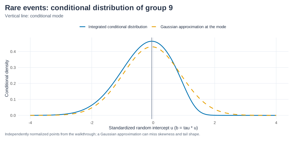
Use increasing node counts to assess sensitivity, especially for rare outcomes and small groups. The verification reports errors at each fitted parameter vector; 61 nodes is still an approximation, not an accuracy guarantee for every dataset. fixed_fitted evaluates probabilities at b=0; it is not a population probability averaged over b. fitted uses each group’s conditional mode.
The code is crates/stats-core/src/logistic_mixed.rs. The core owns numeric vectors/matrices and returns Result<LogisticMixedResult, StatsError>. The PHP binding handles original input validation, one shared missing-row mask, group labels and plain-array output. Application fitting does not invoke R or Python.
From phpstats/phit@76b22f0.